Product sales analysis — optimising sales strategies for a new stationery line
The business question
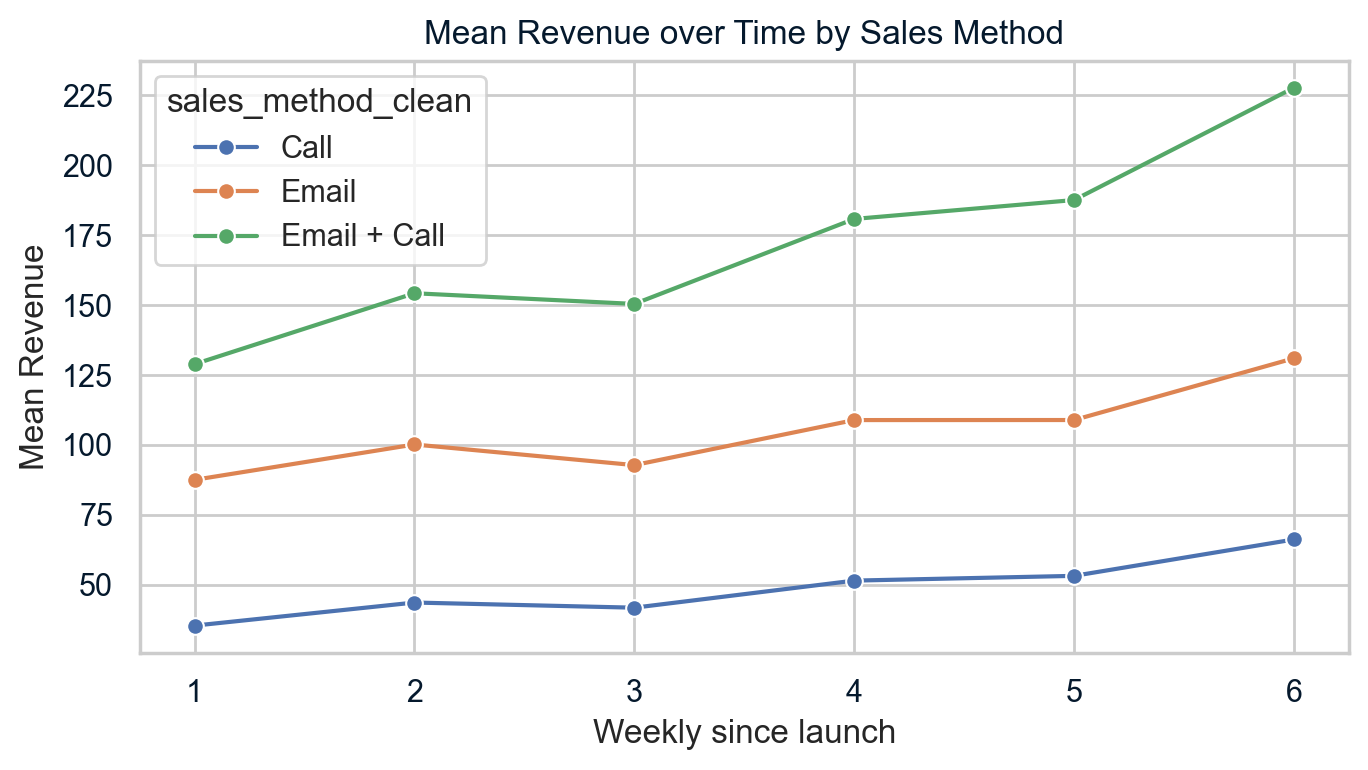
A company launching a new stationery product line ran three sales approaches simultaneously — email only, calls only, and email + call combined. Which strategy delivered the best conversion rate per sales-hour invested?
What I did
Designed and executed an A/B/C statistical test across the three sales cohorts. Calculated conversion rates, revenue per customer, and cost-per-acquisition for each method. Applied hypothesis testing (chi-square) to confirm statistical significance before recommending a winner.
Key finding
The Email + Call strategy produced the highest conversion rate (24% vs 11% email-only), but when adjusted for sales rep time (avg 10 min vs 30 min for call-only), it delivered 3.1x more revenue per hour of effort — making it the clear recommendation for rollout.